Rural Catchments: Difference between revisions
m (remove hierarchy extension template) |
|||
| (36 intermediate revisions by 3 users not shown) | |||
| Line 1: | Line 1: | ||
{{ | {{BlueM.Sim_nav}} | ||
{{BlueMTheory_nav}} | |||
The natural process leading from rain to run-off is divided into three phases. The phases are Belastungsbildung, run-off generation (bzw. Belastungsaufteilung) and run-off concentration. The calculation approach for each of these phases is described in the following sections of this article. | |||
==Belastungsbildung== | ==Belastungsbildung== | ||
== | Die Belastungsbildung describes the determination of an areal rainfall for the considered catchment.Rainfall data is imported into BlueM via external time series. Therefore no explicit calculations are necessary for this phase. | ||
==Run-off generation== | |||
In this phase surface run-off, infiltration, evaporation and interflow are determined by calculating the effective rainfall out of the fallen rain. Snow is calculated for temperatures below 0°C. The Snow-Compaction-Method {{:Literatur:Knauf_1980|Knauf}} is applied. | |||
Rainfall (system load) is divided into rainfall which directly generates run-off and run-off diminishing losses (wetting, trough, evaporation and infiltration losses). Therefore this phase is also called the Belastungsaufteilung. The mathematical equation for the momentary Belastungsaufteilung is as follows: | |||
:<math>Nw(t) = N(t) - VP(t) - I(t) - \frac{dO}{dt} - \frac{dS}{dt}</math> | :<math>Nw(t) = N(t) - VP(t) - I(t) - \frac{dO}{dt} - \frac{dS}{dt}</math> | ||
:mit: | :mit: | ||
:NW = | :NW = run-off generating rainfall | ||
:N = | :N = rainfall | ||
:VP = | :VP = potential evaporation | ||
:I = | :I = infiltration into the soil | ||
:O = | :O = surfacce water reservoir content | ||
:S = | :S = snow reservoir content | ||
The individual elements of the equation and the calculation of these elements is described in the following. | |||
===Rainfall N(t)=== | |||
BlueM requires rainfall data in form of rain time series. In general is does not matter if a block rain, Regenspektrum or a longtime rainfall time series. Depending on the purpose of the simulation the appropriate load (type) must be chosen. Rainfall time series originate out of the BlueM time series management <span class="TALSIM"> or are created immediately before simulation begin as is the case for short term prediction by supplying a rainfall duration, rainfall height and choosing a model rainfall </span>. | |||
====a) | |||
[[ | ===Evaporation VP(t)=== | ||
There are two possibilities for the [[EZG-Datei|input]] of potential evaporation: | |||
====a) annual evaporation ==== | |||
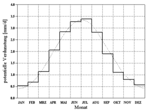
[[File:Theorie_Abb33.gif|thumb|Abbildung 33: annual pattern of potential evaporation according to {{:Literatur:Brandt_1979}}]] | |||
A normed annual pattern of potential evaporation according to {{:Literatur:Brandt_1979|Brandt}} is utilized for the calculation of potential evaporation. Through the evaluation of measurements from twenty different stations, whichs mean-values are depicted as a histogram in [[:File:Theorie_Abb33.gif|Abbildung 33]], the following smoothing function was derived (doted line in [[:File:Theorie_Abb33.gif|Abbildung 33]]): | |||
:<math>VP[\mbox{mm/d}] = \begin{cases}(0.96 + 0.0033 \cdot i) \cdot \sin(\frac{2 \pi}{365})(i - 148) + 1.58, & i <= 300 \\ 2.56 - 1.53 / 65. \cdot (i - 300.), & i > 300 \end{cases}</math> | :<math>VP[\mbox{mm/d}] = \begin{cases}(0.96 + 0.0033 \cdot i) \cdot \sin(\frac{2 \pi}{365})(i - 148) + 1.58, & i <= 300 \\ 2.56 - 1.53 / 65. \cdot (i - 300.), & i > 300 \end{cases}</math> | ||
: | :´with | ||
:i = | :i = ongoing day of the hydrological year | ||
:i = 1 → 1. November | :i = 1 → 1. November | ||
Potential evaporation according to Brandt refers to {{:Literatur:DVWK_1996|'''grass reference evaporation'''}} and assumes an annual total evaporation loss of 654,282 mm. If a different annual total evaporation loss is entered, the value determined by Brandt is scaled accordingly. | |||
==== | ====b) evaporation time series==== | ||
If a evaporation time series is supplied the utilized time step is imported. <br/> | |||
''Attention:'' For time steps < 1 day the time series value is additionally overprinted with a daily pattern! (Bug 1) | |||
=== | ====daily pattern of evaporation==== | ||
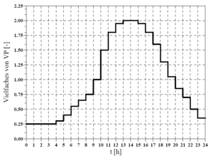
[[File:Theorie_Abb34.gif|thumb|Abbildung 34: Daily pattern of potential evaporation as a multiple of mean daily evaporation]] | |||
If the chosen time step for the calculation is < 1 day the potential evaporation for each time step is calculated by taking the daily pattern depicted in [[:File:Theorie_Abb34.gif|Abbildung 34]] into consideration. If the chosen time step is ≥ 1 day the daily pattern is disregarded. | |||
===Surface water reservoir content(fraction of impervious area) O=== | |||
Snow reservoir content as well as infiltration can be neglected for impervious areas. Therefore the equation of balance is reduced to: | |||
:<math>Nw(t) = N(t) - VP(t) - \frac{dO}{dt}</math> | :<math>Nw(t) = N(t) - VP(t) - \frac{dO}{dt}</math> | ||
in which the change in surface water reservoir content <code>dO/dt</code> represents wetting of the surface as well as filling and depletion of water (through evaporation) in troughs. | |||
The wetting loss (BV) for impervious areas is set to the following standard value. | |||
:<code>BV = 0.5 mm</code> | :<code>BV = 0.5 mm</code> | ||
Trough loss (MV) is set by the user in the [[ALL-Datei|ALL-File]]. | |||
[[ | |||
The trough loss is the mean value for an inclined surface. Due to the fact that troughs are not evenly distributed and experience has shown that run-off occurs before all troughs are completely filled the following assumption is made, that: | |||
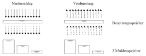
[[File:Theorie_Abb35.gif|thumb|Abbildung 35: Schematic of the model approach for wetting and trough losses]] | |||
* 1/3 of the impervious area has a reduced trough loss of 1/3 MV | |||
* 1/3 of the impervious area has a mean trough loss of 3/3 MV | |||
* 1/3 of the impervious area has a elevated trough loss of 5/3 MV | |||
. Therefore run-off occurs as soon as the rainfall (reduced by evaporation) is greater than wetting losses and 1/3 of the trough losses (in dry antecedent conditions). In [[:File:Theorie_Abb35.gif|Abbildung 35]] the assumptions are depicted schematically. | |||
The run-off coefficient of the impervious areas (after overcoming initial losses) is set to ψ = 1. When determining the fraction of impervious areas for a catchment it needs to be considered that not all paved or impervious areas drain into the canalization. | |||
Wetting and trough losses are continuously made available through the ongoing balancing of these reservoirs and evaporation. | |||
===Surface water reservoir content (fraction of pervious areas) O=== | |||
Surface water reservoir content is determined through the ongoing balancing of a loss reservoir in dependency of the chosen run-off generation approach.Details can be found in the following sections about calculation of infiltration respectively run-off generating rainfall. | |||
===Infiltration respectively run-off generating rainfall I(t), Nw(t)=== | |||
Infiltration into the soil can not be neglected for pervious areas due to the fact that infiltration substantially influences run-off. Three approaches were implemented in the model for the calculation of infiltration: | |||
# constant run-off coefficient ψ | |||
# event specific run-off coefficient similar to the method of the Soil-Conservation-Service (SCS) | |||
# soil moisture simulation | |||
====constant run-off coefficient ψ==== | |||
By supplying a ψ<sub>u</sub>-value the remaining rainfall after having covered the initial losses (wetting and trough losses)generates run-off according to the ratio of the run-off coefficient ψ<sub>u</sub> independent of previous history and the characteristics of the rainfall (height, intensity, duration). If possible this approach should not be used, because it only represents a very rudimentary description of the run-off generation process. | |||
====SCS-Method==== | |||
:''refer to [[SCS-Verfahren|SCS-Method]]'' | |||
[[ | ====Soil moisture simulation==== | ||
:''refer to [[Bodenfeuchtesimulation|Soil moisture simulation]]'' | |||
==Run-off concentration== | |||
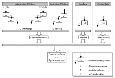
[[File:Parallelspeicherkaskade_EZG.gif|thumb|400px|Abbildung 44: Calculation of run-off concentration for rural catchments]] | |||
Run-off concentration determines the delay of discharge out of the catchment. Calculation of Interflow and base flow is dependent on the chosen calculation approach. If [[Bodenfeuchteberechnung|soil moisture simulation]] is chosen, the discharge of both run-off components at the catchment outlet is delayed through a linear reservoir. If the run-off coefficient approach or the SCS-Method is chosen, interflow is neglected and base flow is determined through regarding the given specific base discharge and a possible consideration of an annual pattern. | |||
A parallel reservoir cascade is utilized with two reservoirs each for the cascade for pervios and the cascade for impervious areas. | |||
The reservoir cascades can be calculated as linear or [[Speicherbaustein|non-linear reservoirs]]. If the reservoir cascade parameters are not supplied, they are calculated through using area characteristics according to {{:Literatur:Zaiß 1986}} | |||
==Literature== | |||
== | |||
<references/> | <references/> | ||
[[Category:BlueM Theorie]] | |||
[[ | |||
Latest revision as of 07:37, 9 January 2015
![]() BlueM.Sim | Download | Application | Theory | Development
BlueM.Sim | Download | Application | Theory | Development
BlueM.Sim theory
The natural process leading from rain to run-off is divided into three phases. The phases are Belastungsbildung, run-off generation (bzw. Belastungsaufteilung) and run-off concentration. The calculation approach for each of these phases is described in the following sections of this article.
Belastungsbildung
Die Belastungsbildung describes the determination of an areal rainfall for the considered catchment.Rainfall data is imported into BlueM via external time series. Therefore no explicit calculations are necessary for this phase.
Run-off generation
In this phase surface run-off, infiltration, evaporation and interflow are determined by calculating the effective rainfall out of the fallen rain. Snow is calculated for temperatures below 0°C. The Snow-Compaction-Method Knauf[1] is applied.
Rainfall (system load) is divided into rainfall which directly generates run-off and run-off diminishing losses (wetting, trough, evaporation and infiltration losses). Therefore this phase is also called the Belastungsaufteilung. The mathematical equation for the momentary Belastungsaufteilung is as follows:
- [math]\displaystyle{ Nw(t) = N(t) - VP(t) - I(t) - \frac{dO}{dt} - \frac{dS}{dt} }[/math]
- mit:
- NW = run-off generating rainfall
- N = rainfall
- VP = potential evaporation
- I = infiltration into the soil
- O = surfacce water reservoir content
- S = snow reservoir content
The individual elements of the equation and the calculation of these elements is described in the following.
Rainfall N(t)
BlueM requires rainfall data in form of rain time series. In general is does not matter if a block rain, Regenspektrum or a longtime rainfall time series. Depending on the purpose of the simulation the appropriate load (type) must be chosen. Rainfall time series originate out of the BlueM time series management or are created immediately before simulation begin as is the case for short term prediction by supplying a rainfall duration, rainfall height and choosing a model rainfall .
Evaporation VP(t)
There are two possibilities for the input of potential evaporation:
a) annual evaporation

A normed annual pattern of potential evaporation according to Brandt[2] is utilized for the calculation of potential evaporation. Through the evaluation of measurements from twenty different stations, whichs mean-values are depicted as a histogram in Abbildung 33, the following smoothing function was derived (doted line in Abbildung 33):
- [math]\displaystyle{ VP[\mbox{mm/d}] = \begin{cases}(0.96 + 0.0033 \cdot i) \cdot \sin(\frac{2 \pi}{365})(i - 148) + 1.58, & i \lt = 300 \\ 2.56 - 1.53 / 65. \cdot (i - 300.), & i \gt 300 \end{cases} }[/math]
- ´with
- i = ongoing day of the hydrological year
- i = 1 → 1. November
Potential evaporation according to Brandt refers to grass reference evaporation[3] and assumes an annual total evaporation loss of 654,282 mm. If a different annual total evaporation loss is entered, the value determined by Brandt is scaled accordingly.
b) evaporation time series
If a evaporation time series is supplied the utilized time step is imported.
Attention: For time steps < 1 day the time series value is additionally overprinted with a daily pattern! (Bug 1)
daily pattern of evaporation
If the chosen time step for the calculation is < 1 day the potential evaporation for each time step is calculated by taking the daily pattern depicted in Abbildung 34 into consideration. If the chosen time step is ≥ 1 day the daily pattern is disregarded.
Surface water reservoir content(fraction of impervious area) O
Snow reservoir content as well as infiltration can be neglected for impervious areas. Therefore the equation of balance is reduced to:
- [math]\displaystyle{ Nw(t) = N(t) - VP(t) - \frac{dO}{dt} }[/math]
in which the change in surface water reservoir content dO/dt represents wetting of the surface as well as filling and depletion of water (through evaporation) in troughs.
The wetting loss (BV) for impervious areas is set to the following standard value.
BV = 0.5 mm
Trough loss (MV) is set by the user in the ALL-File.
The trough loss is the mean value for an inclined surface. Due to the fact that troughs are not evenly distributed and experience has shown that run-off occurs before all troughs are completely filled the following assumption is made, that:
- 1/3 of the impervious area has a reduced trough loss of 1/3 MV
- 1/3 of the impervious area has a mean trough loss of 3/3 MV
- 1/3 of the impervious area has a elevated trough loss of 5/3 MV
. Therefore run-off occurs as soon as the rainfall (reduced by evaporation) is greater than wetting losses and 1/3 of the trough losses (in dry antecedent conditions). In Abbildung 35 the assumptions are depicted schematically.
The run-off coefficient of the impervious areas (after overcoming initial losses) is set to ψ = 1. When determining the fraction of impervious areas for a catchment it needs to be considered that not all paved or impervious areas drain into the canalization.
Wetting and trough losses are continuously made available through the ongoing balancing of these reservoirs and evaporation.
Surface water reservoir content (fraction of pervious areas) O
Surface water reservoir content is determined through the ongoing balancing of a loss reservoir in dependency of the chosen run-off generation approach.Details can be found in the following sections about calculation of infiltration respectively run-off generating rainfall.
Infiltration respectively run-off generating rainfall I(t), Nw(t)
Infiltration into the soil can not be neglected for pervious areas due to the fact that infiltration substantially influences run-off. Three approaches were implemented in the model for the calculation of infiltration:
- constant run-off coefficient ψ
- event specific run-off coefficient similar to the method of the Soil-Conservation-Service (SCS)
- soil moisture simulation
constant run-off coefficient ψ
By supplying a ψu-value the remaining rainfall after having covered the initial losses (wetting and trough losses)generates run-off according to the ratio of the run-off coefficient ψu independent of previous history and the characteristics of the rainfall (height, intensity, duration). If possible this approach should not be used, because it only represents a very rudimentary description of the run-off generation process.
SCS-Method
- refer to SCS-Method
Soil moisture simulation
- refer to Soil moisture simulation
Run-off concentration
Run-off concentration determines the delay of discharge out of the catchment. Calculation of Interflow and base flow is dependent on the chosen calculation approach. If soil moisture simulation is chosen, the discharge of both run-off components at the catchment outlet is delayed through a linear reservoir. If the run-off coefficient approach or the SCS-Method is chosen, interflow is neglected and base flow is determined through regarding the given specific base discharge and a possible consideration of an annual pattern.
A parallel reservoir cascade is utilized with two reservoirs each for the cascade for pervios and the cascade for impervious areas. The reservoir cascades can be calculated as linear or non-linear reservoirs. If the reservoir cascade parameters are not supplied, they are calculated through using area characteristics according to Zaiß (1986)[4]
Literature
- ↑ Knauf, D. (1980): Die Berechnung des Abflusses aus einer Schneedecke, in: DVWK-Schriften, Heft 46, Analyse und Berechnung oberirdischer Abflüsse PDF

- ↑ 2.0 2.1 Brandt, T. (1979): Modell zur Abflussgangliniensimulation unter Berücksichtigung des grundwasserbürtigen Abflusses, Technischer Bericht Nr. 24 aus dem Institut für Wasserbau, Fachgebiet Ingenieurhydrologie und Hydraulik der TH Darmstadt
- ↑ DVWK (Hrsg.) (1996): Ermittlung der Verdunstung von Land- und Wasserflächen, DVWK-Merkblätter zur Wasserwirtschaft, Heft 238. Bonn: Wirtschafts- und Verlagsgesellschaft Gas und Wasser mbH
- ↑ Zaiß, H. (1986): Abflussermittlung aus Teilflächen, in "Hydrologische Abflussmodelle in der praktischen Anwendung", 36. Fortbildungslehrgang des BWK-Hessen am 21. März 1986, Friedberg [ihwb-Bibliothek: Inv.-Nr. 5593, 10 BWK 36] PDF
 OCR
OCR 


