SensiPlot

BlueM.Opt | Usage | Development

Screenshot of a SensiPlot run with two parameters

Description

SensiPlot is not an optimization algorithm but instead can be used to carry out a sensitivity analysis by varying one or more optimization parameters and analyzing the resulting objective function values.

Required input files

same as with PES

Usage

Example of different parameter sampling modes for two parameters

1. Select an App, a Dataset and then select "SensiPlot" as the Method.
2. Select one or more Optimization parameters to vary.
3. Select an Objective function to show in the main diagram.
4. Select a Mode:
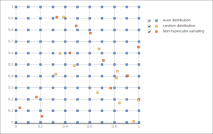
   • Randomly distributed: Each parameter combination is completely random
   • Evenly distributed: All possible parameter combinations are tested (requires nsteps ^ nparams simulations!)
   • Latin Hypercube Sampling: Uses Latin hypercube sampling to generate a near-random sample of parameter values that attempts to cover the entire parameter space.
5. Set the No. of steps: Number of different values to test for each parameter.
6. The option Show time series in Wave will display all simulation results in BlueM.Wave once the SensiPlot run is finished.
7. The option Save individual datasets causes each indivual dataset to be simulated in a subfolder of the original dataset named sensiplot_X, where X is the solution ID. If this option is deactivated, the dataset modifications and simulations are carried out using the original dataset.

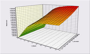
The main diagram will only show up to two optimization parameters and the one selected objective function. To see the values of other optimization parameters and objective functions, use the scatterplot and custom plot features (buttons in the toolbar).

Notes

• Optimization parameters that are not selected will be set to their start values as defined in the OPT-file.
• Constraints are currently not considered (#177)